Examples
Note
This is thrown together quickly to help people have some idea of how to use the work-in-progress release for the QSSC poster. More polish to come in the future.
Note
One needs the superspinsim, numpy, and matplotlib packages to use these examples.
Qubit
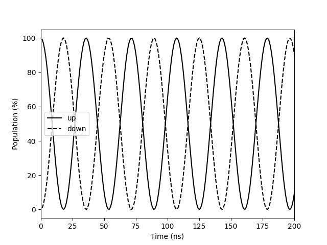
Basic coupling
Our first example simulates a qubit under coupling between its two states. The coupling is given in actual physical units: it has the electron g factor of two, and a magnetic field in the x direction of 1 mT.
import numpy as np
from matplotlib import pyplot as plt

from superspinsim import simspins


# Define magnetic field (constant 1 mT along x)
def mag_x(time):
    return 1e-3

def mag_y(time):
    return 0.0

def mag_z(time):
    return 0.0

# Relevent only for defects
def excitation(time):
    return 0.0

# Define qubit (spin-half, electron g factor)
spins = [[{"S": 1/2, "g": 2.0}]]

# Define density matrix
density_initial = np.zeros((2, 2), dtype=np.float64)
density_initial[0, 0] = 1

# Simulate
time, density = simspins(
    [mag_x, mag_y, mag_z, excitation],  # Fields
    0, 100e-6, 1e-9,                    # Time start/stop/step
    spins, [{}], {},                    # Spin description
    density_initial                     # Initial state
)

# Plot
plt.figure(label="Lab frame")
plt.plot(time/1e-9, density[:, 0, 0].real/1e-2, "k-", label="up")
plt.plot(time/1e-9, density[:, 1, 1].real/1e-2, "k--", label="down")
plt.xlim(0, 200)
plt.xlabel("Time (ns)")
plt.ylabel("Population (%)")
plt.legend()
Expected output:
Though this is a basic illustrative example, it is not the recommended way of simulating a constant bias field in SuperSpinsim. If we know that the dynamics are dominated by (or entirely) a DC bias term, then it is more efficient to diagonalise the problem and work within a “generalised rotating frame”. To use this, define a bias magnetic field in the definition of the spin system.
Note
This is not the same as using the rotating wave approximation. The simulator makes no approximations here and actually improves precision.
import numpy as np
from matplotlib import pyplot as plt

from superspinsim import simspins

# No "interaction" magnetic field
def mag_x(time):
    return 0.0

def mag_y(time):
    return 0.0

def mag_z(time):
    return 0.0

# Relevent only for defects
def excitation(time):
    return 0.0

# Define qubit
spins = [[{
    "S": 1/2, "g": 2.0,           # (spin-half, electron g factor)
    "B0": np.array([1e-3, 0, 0])  # Bias magnetic field of 1 mT along x
}]]

# Define density matrix
density_initial = np.zeros((2, 2), dtype=np.float64)
density_initial[0, 0] = 1

# Simulate
time, density = simspins(
    [mag_x, mag_y, mag_z, excitation],  # Fields
    0, 100e-6, 1e-9,                    # Time start/stop/step
    spins, [{}], {},                    # Spin description
    density_initial                     # Initial state
)

# Plot
plt.figure(label="Rotating frame")
plt.plot(time/1e-9, density[:, 0, 0].real/1e-2, "k-", label="up")
plt.plot(time/1e-9, density[:, 1, 1].real/1e-2, "k--", label="down")
plt.xlim(0, 200)
plt.xlabel("Time (ns)")
plt.ylabel("Population (%)")
plt.legend()
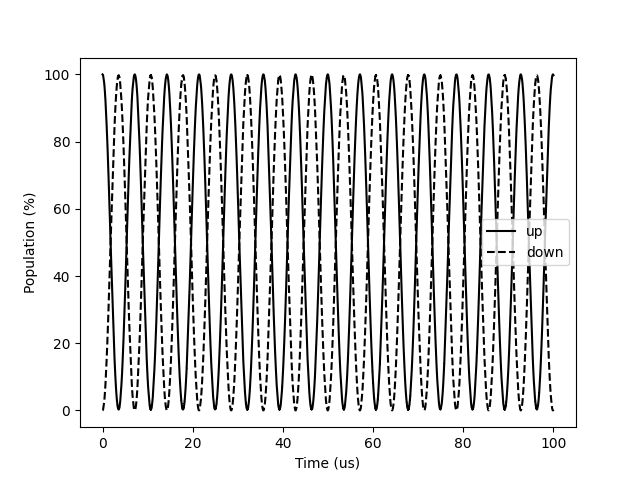
Rabi problem
We can use time-dependent fields to solve the Rabi problem.
import math
import numpy as np
from matplotlib import pyplot as plt

from superspinsim import simspins

# Define magnetic field (Rabi dressing)
dressing_frequency = 28e6   # ~ on resonance
dressing_amplitude = 10e-6  # 10 uT

def mag_x(time):
    return dressing_amplitude*math.cos(math.tau*dressing_frequency*time)

def mag_y(time):
    return 0.0

def mag_z(time):
    return 0.0

# Relevent only for defects
def excitation(time):
    return 0.0

# Define qubit
spins = [[{
    "S": 1/2, "g": 2.0,           # (spin-half, electron g factor)
    "B0": np.array([0, 0, 1e-3])  # Bias magnetic field of 1 mT along z
}]]

# Define density matrix
density_initial = np.zeros((2, 2), dtype=np.float64)
density_initial[0, 0] = 1

# Simulate
time, density = simspins(
    [mag_x, mag_y, mag_z, excitation],  # Fields
    0, 100e-6, 1e-9,                    # Time start/stop/step
    spins, [{}], {},                    # Spin description
    density_initial                     # Initial state
)

# Plot
plt.figure(label="Rabi problem")
plt.plot(time/1e-6, density[:, 0, 0].real/1e-2, "k-", label="up")
plt.plot(time/1e-6, density[:, 1, 1].real/1e-2, "k--", label="down")
plt.xlabel("Time (us)")
plt.ylabel("Population (%)")
plt.legend()
Expected output:
NV systems
SuperSpinsim contains a model for the nitrogen-vacancy (NV) centre in diamond. Specifically, this is the seven level model of optical transitions and spin dynamics. This is just a predefined spin description (see API) defining interactions within and between the NV orbitals.
Note
The NV plots use the colour maps from cmcrameri.
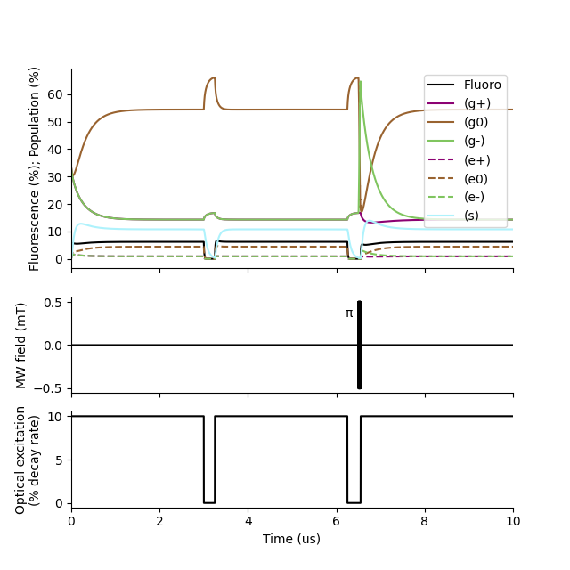
Contrast experiment
A standard constrast experiment on an NV centre. We look at the fluorescence response of the NV as it is excited from a thermal state, a polarised mS = 0 state, and a polarised mS = -1 state. The difference between the response in the last two can be used to determine spin projection from fluorescence at the end of future experiments.
Here, fluorescence is modelled as the population of the excited state, since it is proportional to that.
We also include an illustrative plotting script to show what is happening during the experiment.
import math
import numpy as np
from matplotlib import pyplot as plt
from cmcrameri import cm

from superspinsim import simspins
from superspinsim.models import nv_7

# Define pulse sequence
duration_excitation = 3e-6
duration_relax_wait = 250e-9
duration_mw = 1/(2*10e6)
frequency_mw = 2.87e9 - 280e6
amplitude_mw = math.sqrt(1/2)*2*10e6/28e9
excitation_amplitude = 0.1

time_thermal_start = 0
time_thermal_end = time_thermal_start + duration_excitation
time_zero_start = duration_excitation + duration_relax_wait
time_zero_end = time_zero_start + duration_excitation
time_one_start = 2*duration_excitation + 2*duration_relax_wait \
    + duration_mw
time_one_end = time_one_start + duration_excitation
time_end = 10e-6

time_start = 0
time_step = 1e-9

bias_field = np.array([0, 0, 1])*10e-3

def mag_x(time):
    if time < time_one_start - duration_mw:
        return 0
    if time < time_one_start:
        return amplitude_mw*math.sin(math.tau*frequency_mw*time)
    return 0

def mag_y(time):
    return 0

def mag_z(time):
    return 0

def excitation(time):
    if time < time_thermal_end:
        return excitation_amplitude
    if time < time_zero_start:
        return 0
    if time < time_zero_end:
        return excitation_amplitude
    if time < time_one_start:
        return 0
    return excitation_amplitude

# Initial state (thermal in ground orbital state)
density_initial = np.zeros((7, 7), dtype=np.float64)
density_initial[0, 0] = 1/3
density_initial[1, 1] = 1/3
density_initial[2, 2] = 1/3

# Define model
model = nv_7(bias_field)

# Simulate
time, density = simspins(
    [mag_x, mag_y, mag_z, excitation],
    time_start, time_end, time_step,
    *model,
    density_initial
)

# Get fluorescence
fluorescence = density[:, 3, 3] + density[:, 4, 4] + density[:, 5, 5]
fluorescence = fluorescence.real

# Plot
time_coefficients_sample = np.arange(time_start, time_end, time_step/10)
coefficient_sample_x = np.empty_like(time_coefficients_sample)
coefficient_sample_l = np.empty_like(time_coefficients_sample)
for time_index, time_sample in enumerate(time_coefficients_sample):
    coefficient_sample_x[time_index] = mag_x(time_sample)
    coefficient_sample_l[time_index] = excitation(time_sample)

plt.figure(
    label="fluorescence",
    figsize=(6.4, 6.4)
)
plt.subplot(2, 1, 1)
plt.plot(time/1e-6, fluorescence/0.01, "k-", label="Fluoro")
plt.plot(
    time/1e-6, np.real(density[:, 0, 0])/0.01, "-", color=cm.hawaii(0/3),
    label="(g+)"
)
plt.plot(
    time/1e-6, np.real(density[:, 1, 1])/0.01, "-", color=cm.hawaii(1/3),
    label="(g0)"
)
plt.plot(
    time/1e-6, np.real(density[:, 2, 2])/0.01, "-", color=cm.hawaii(2/3),
    label="(g-)"
)
plt.plot(
    time/1e-6, np.real(density[:, 3, 3])/0.01, "--", color=cm.hawaii(0/3),
    label="(e+)"
)
plt.plot(
    time/1e-6, np.real(density[:, 4, 4])/0.01, "--", color=cm.hawaii(1/3),
    label="(e0)"
)
plt.plot(
    time/1e-6, np.real(density[:, 5, 5])/0.01, "--", color=cm.hawaii(2/3),
    label="(e-)"
)
plt.plot(
    time/1e-6, np.real(density[:, 6, 6])/0.01, "-", color=cm.hawaii(0.99),
    label="(s)"
)
plt.xlim(0, time_end/1e-6)
plt.ylabel("Fluorescence (%); Population (%)")
plt.legend()
plt.gca().set_xticklabels([])
plt.gca().spines[["top", "right"]].set_visible(False)

plt.subplot(4, 1, 3)
plt.plot(time_coefficients_sample/1e-6, coefficient_sample_x/1e-3, "k-")
plt.text(6.2, 0.3, "π", va="bottom")
plt.xlim(0, time_end/1e-6)
plt.ylabel("MW field (mT)")
plt.gca().set_xticklabels([])
plt.gca().spines[["top", "right"]].set_visible(False)

plt.subplot(4, 1, 4)
plt.plot(time_coefficients_sample/1e-6, coefficient_sample_l/1e-2, "k-")
plt.xlim(0, time_end/1e-6)
plt.xlabel("Time (us)")
plt.ylabel("Optical excitation\n(% decay rate)")
plt.gca().spines[["top", "right"]].set_visible(False)
Expected output:
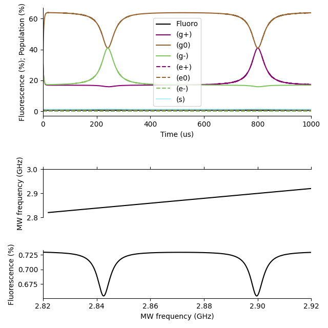
ODMR
This ODMR sweep has a fully-rendered microwave tone.
# Define pulse sequence
time_start = 1e-6
time_end = 1000e-6
time_step = 150e-9
frequency_start = 2.82e9
frequency_width = 100e6

bias_field = np.array([0, 0, 1])*1e-3

def mag_x(time):
    if time > time_start:
        phase = math.tau*(
            frequency_start*(time - time_start)
            + frequency_width*((time - time_start)**2)
            / (time_end - time_start)/2
        )
        return 100e-6*math.sin(phase)
    else:
        return 0

def mag_y(time):
    return 0

def mag_z(time):
    return 0

def excitation(time):
    return 0.01

# Initial state (thermal in ground orbital state)
density_initial = np.zeros((7, 7), dtype=np.float64)
density_initial[0, 0] = 1/3
density_initial[1, 1] = 1/3
density_initial[2, 2] = 1/3

# Define model
model = nv_7(bias_field)

# Simulate
time, density = simspins(
    [mag_x, mag_y, mag_z, excitation],
    0, time_end, time_step,
    *model,
    density_initial,
    # Integrate on a finer time step than is output
    number_of_fine_divisions=300
)

# Get fluorescence
fluorescence = density[:, 3, 3] + density[:, 4, 4] + density[:, 5, 5]
fluorescence = fluorescence.real

# Plot
plt.figure(
    label="fluorescence",
    figsize=(6.4, 6.4)
)
plt.subplot(2, 1, 1)
plt.plot(time/1e-6, fluorescence/0.01, "k-", label="Fluoro")
plt.plot(
    time/1e-6, np.real(density[:, 0, 0])/0.01, "-", color=cm.hawaii(0/3),
    label="(g+)"
)
plt.plot(
    time/1e-6, np.real(density[:, 1, 1])/0.01, "-", color=cm.hawaii(1/3),
    label="(g0)"
)
plt.plot(
    time/1e-6, np.real(density[:, 2, 2])/0.01, "-", color=cm.hawaii(2/3),
    label="(g-)"
)
plt.plot(
    time/1e-6, np.real(density[:, 3, 3])/0.01, "--", color=cm.hawaii(0/3),
    label="(e+)"
)
plt.plot(
    time/1e-6, np.real(density[:, 4, 4])/0.01, "--", color=cm.hawaii(1/3),
    label="(e0)"
)
plt.plot(
    time/1e-6, np.real(density[:, 5, 5])/0.01, "--", color=cm.hawaii(2/3),
    label="(e-)"
)
plt.plot(
    time/1e-6, np.real(density[:, 6, 6])/0.01, "-", color=cm.hawaii(0.99),
    label="(s)"
)
plt.xlim(0, time_end/1e-6)
plt.xlabel("Time (us)")
plt.ylabel("Fluorescence (%); Population (%)")
plt.legend()
plt.gca().spines[["top", "right"]].set_visible(False)

time_start = 1e-6
frequency_start = 2.82e9
frequency_width = 100e6
mw_frequency = frequency_start \
    + frequency_width*(time - 20*time_start)/(time_end - 20*time_start)
mw_frequency = mw_frequency[time > 20*time_start]
clipped_odmr = fluorescence[time > 20*time_start]

plt.subplot(4, 1, 3)
plt.plot(time[time > 20*time_start]/1e-6, mw_frequency/1e9, "k-")
plt.gca().set_xticklabels([])
plt.xlim(0, time_end/1e-6)
plt.ylim(2.8, 3)
plt.ylabel("MW frequency (GHz)")
plt.gca().spines[["bottom", "right"]].set_visible(False)
plt.gca().xaxis.tick_top()

plt.subplot(4, 1, 4)
plt.plot(mw_frequency/1e9, clipped_odmr/1e-2, "k-")
plt.xlim(frequency_start/1e9, (frequency_start + frequency_width)/1e9)
plt.xlabel("MW frequency (GHz)")
plt.ylabel("Fluorescence (%)")
plt.gca().spines[["top", "right"]].set_visible(False)

plt.tight_layout()
Expected output: